多个弱学习器，组成1个强学习器的过程

三个裨将赛过诸葛亮

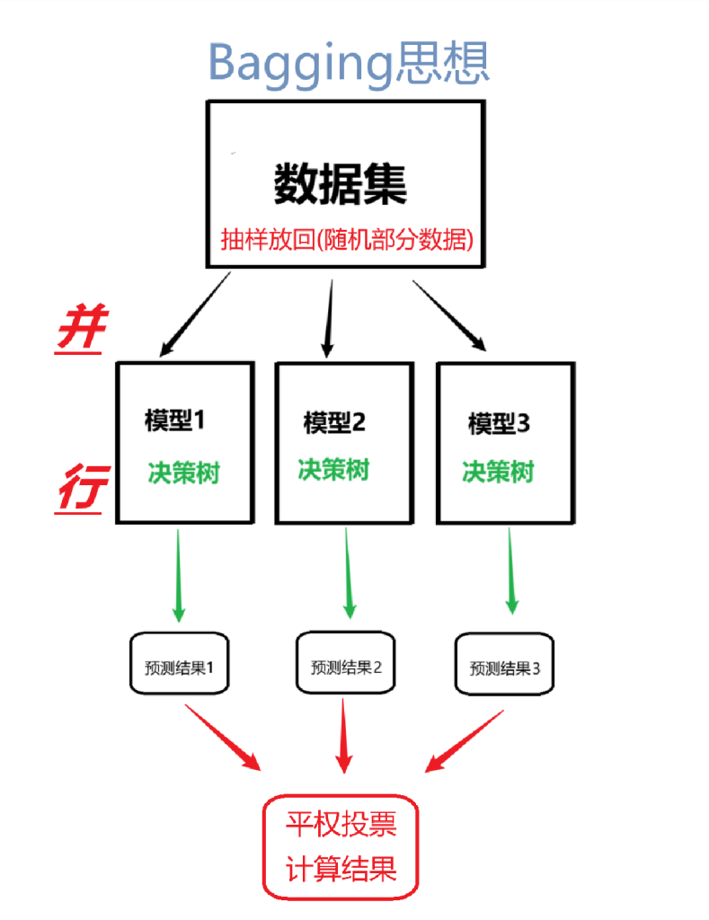
Bagging思想

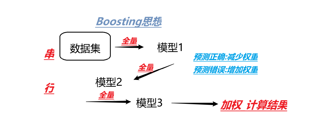
Boosting思想

随机森林(分类首选基线模型)


Bagging思想 
sklearn.ensemble.RandomForestClassifier() 
基线模型->第一版能跑通的模型
n_estimators: 决策树数量
Criterion: entropy(增益)或者gini(默认)
max_depth:指定最大深度
max_features="auto",决策树构建时使用的最大特征数量
auto参 √number
sqrt: 同上
log2: log2(number)
bootstrap:是否采用有放回抽样default=True

min_imputity_split:2023后过时

以下全是Boosting思想

Adaboost(自适应决策树)

auto决策树

模型权重与错误率

`如何推导？`

构建n棵弱学习器，计算错误率，模型权重，以及更新后的样本权重

各个预测样本在各个决策树中计算模型权重*各个预测的分类的累加和

如果 >0 则：正例否则：反例

代码示例

import pandas as pd
from sklearn.preprocessing import LabelEncoder
from sklearn.model_selection import train_test_split
from sklearn.tree import DecisionTreeClassifier
from sklearn.ensemble import AdaBoostClassifier
from sklearn.metrics import accuracy_score
#数据加载
data = pd.read_csv('data/wine0501.csv')
#数据的预处理
    #因为决策树只能做二分类，索引我们从三个类别中，筛选出2，3类别的信息
# data = data[data['Class lable'].isin([2,3])]
data = data[data['Class label'] != 1]
#从伤处数据中筛选出特征数据和标签数据
x = data[['Alcohol','Hue']] #酒精和色泽
y = data['Class label']#标签2，3
#标签数据转换成数值类型的 0，1形式 Str to int
le = LabelEncoder()#标签编码器对象
y = le.fit_transform(y)

x_train,x_test,y_train,y_test=train_test_split(x,y,test_size=0.2,random_state=22,stratify=y)
#特征工程
#模型训练
estimator1 = DecisionTreeClassifier(criterion='gini', max_depth=3)
estimator1.fit(x_train,y_train)
y_pre1 = estimator1.predict(x_test)
print(f'预测值为：{y_pre1}')
print(f'准确率{accuracy_score(y_pre1,y_test)}')

#1:弱学习对象 2：基学习个数 3：学习率 是作用于第一颗树 4：使用说明算法
estimator2 = AdaBoostClassifier(estimator=estimator1,n_estimators=100,learning_rate=1,algorithm="SAMME")
estimator2.fit(x_train,y_train)
y_pre2 = estimator2.predict(x_test)
print(f'预测值为：{y_pre2}')
print(f'准确率{accuracy_score(y_pre2,y_test)}')

GBDT(梯度提升树)

残差 换负梯度

负梯度 = 残差 =目标值的均值(误差平方和 最小-模型就最好)

1、初始化弱学习器(目标值的均值作为预测值)

2、迭代构建学习器，每一个学习器拟合上一个学习器的负梯度

3、直到达到指定的学习器个数

4、当输入位置样本时，将所有弱学习器的输出结果组合起来作为强学习器的输出

结果：

左:-▲(均) = A

右:x1到xn的特征 /x_sum =0.19 =预测值(均)=误差平方和 = B

第一次的预测值是真实值的平均

result = (左树每一个真实值-均值(预测值)+右树每一个真实值-均值(预测值))²

下一轮继续使用result作为真实值把算出来的左子树与右子树当作预测值继续算

最后把树1(真)+树2+树3 =最终结果

代码示例

import pandas as pd
from sklearn.model_selection import train_test_split
from sklearn.tree import DecisionTreeClassifier
from sklearn.ensemble import  GradientBoostingClassifier
from sklearn.metrics import accuracy_score,classification_report
from sklearn.model_selection import GridSearchCV
data = pd.read_csv('data/train.csv')
x = data[['Pclass','Age','Sex']].copy()
y = data['Survived']
# x.Age = x.Age.fillna(x.Age.mean())
x['Age'] = x['Age'].fillna(x['Age'].mean())
x = pd.get_dummies(x,columns=['Sex'])
x_train,x_test,y_train,y_test = train_test_split(x, y, test_size=0.2, random_state=22)
#
# # print(x.head())


estimator1 = GradientBoostingClassifier()
estimator1.fit(x_train,y_train)
y_pre = estimator1.predict(x_test)
param_grid = {"n_estimators":[100,200],"learning_rate":[0.1,0.2],"max_depth":[3,5]}
best_estimator2 = GridSearchCV(estimator1,param_grid,cv=4)
best_estimator2.fit(x_train,y_train)
pre2 = best_estimator2.predict(x_test)
print(accuracy_score(y_test,pre2))

XGBoost(极端梯度提升树)

极端 ▲提升

损失函数 + 正则化(控制每个弱学习的复杂程度，叶子节点数和树输出的结果)

泰勒展开：二阶，使用t-1个弱学习器构成的继承模型损失求解当前t个弱学习的损失

角度转换：同意将样本的计算转换树的角度

判断一个树是否要进行分类

step1:初始XGboost的目标函数损失函数+正则化

step2:基于泰勒展开二阶式进行转换，转成近似函数

step3:把问题从样本角度--> 叶子节点角度进行分析

step4:得到最终结论，打分函数

推导过程：

目标函数：损失函数 + 正则化Obj = Σ L(yᵢ, ŷᵢ) + Σ Ω(fₖ)
泰勒二阶展开 近似损失函数
合并同叶子节点样本，对 w 求导得最优权重：wⱼ* = -Gⱼ/(Hⱼ+λ)（Gⱼ为叶子节点一阶梯度之和，Hⱼ为二阶梯度之和，λ为正则化参数）
代入得结构分数（打分函数）：Obj* = -½ Σ Gⱼ²/(Hⱼ+λ) + γT

代码示例

"""
案例:
    演示下XGBoost的用法.

XGBoost介绍:
    概述:
        全称叫 Extreme Gradient Boosting, 极端梯度提升树, 采用 打分函数 的思路进行分枝的.
    原理:
        打分函数(Gain值) = 拆分前 - (拆分左子树 + 拆分后右子树)
        如果Gain值 > 0, 说明拆会后损失函数较小, 可以考虑分裂.
        如果是负数, 说明拆分后损失函数较大, 不适合分裂.
    大白话解释推导过程:
        1. 构建XGBoost的目标函数, 基于: 损失函数 + 正则化(和叶子节点数量, 值有关系)
        2. 基于泰勒二阶展开式获取上述函数的 近似函数.
        3. 把样本角度 -> 转成叶节点角度 做分析.
        4. 得到打分函数.
"""

# 导包
import joblib                   # 保存和加载模型的
import numpy as np              # 数组和矩阵运算
import pandas as pd             # 数据处理
import xgboost as xgb           # XGBoost(极端梯度提升树)模型
from collections import Counter # 统计数据(查看数据分布情况的)
from sklearn.model_selection import train_test_split, GridSearchCV  # 训练集和测试集的划分, 网格搜索对象
from sklearn.metrics import classification_report       # 模型评估(报告)
from sklearn.model_selection import StratifiedKFold     # 分层K折
from sklearn.utils import class_weight                  # (平衡)样本权重


# todo 1. 加载数据.
def dm01_load_data():
    # 1. 加载数据
    data = pd.read_csv('./data/红酒品质分类.csv')
    # print(data.head())
    
    # 2. 抽取特征 和 标签数据.
    x = data.iloc[:, :-1]       # 除了最后一列, 都是特征.
    y = data.iloc[:, -1]        # 最后一列, 是标签.
    # print(x.shape, y.shape)   # (1599, 11) (1599,)

    # 3.对y轴值做处理, 使其从 [3, 8]  -> [0, 5]
    y = y - 3

    # 4. 查看下标签的分布情况.
    print(Counter(y))           # Counter({2: 681, 3: 638, 4: 199, 1: 53, 5: 18, 0: 10}) -> 数据不均衡.

    # 5. 划分训练集和测试集.
    x_train, x_test, y_train, y_test = train_test_split(x, y, test_size=0.2, random_state=27, stratify=y)

    # 6. 把训练集 和 测试集数据, 分别保存到csv文件中.
    # 6.1 把训练集的特征 和 标签保存到csv文件中.
    train_data = pd.concat([x_train, y_train], axis=1)
    train_data.to_csv('./data/红酒品质分类_训练集.csv', index=False)

    # 6.2 把测试集的特征 和 标签保存到csv文件中.
    test_data = pd.concat([x_test, y_test], axis=1)
    test_data.to_csv('./data/红酒品质分类_测试集.csv', index=False)
    print('保存数据成功!')


# todo 2.模型训练并保存.
def dm02_train_model():
    # 1. 加载数据
    train_data = pd.read_csv('./data/红酒品质分类_训练集.csv')
    test_data = pd.read_csv('./data/红酒品质分类_测试集.csv')

    # 2. 分别提取训练集 和 测试集的 特征 和 标签数据.
    x_train = train_data.iloc[:, :-1]
    y_train = train_data.iloc[:, -1]
    x_test = test_data.iloc[:, :-1]
    y_test = test_data.iloc[:, -1]

    # 3. 创建模型对象.
    estimator = xgb.XGBClassifier(
        n_estimators=100,       # 决策树(弱学习器)的个数.
        learning_rate=0.1,      # 学习率.
        max_depth=5,            # 树的深度.
        random_state=27,        # 随机数种子.
        objective='multi:softmax',  # 目标函数(损失函数) -> multi:softmax 适合于多分类问题.
    )

    # 4. 模型训练.
    # 4.1 扩展(可选): 平衡样本权重.
    # 参1: 平衡样本权重的类型, 默认是balanced.       参2: 训练集的标签数据.
    class_weight.compute_sample_weight('balanced', y_train)

    # 4.2 具体的训练过程.
    estimator.fit(x_train, y_train)

    # 5. 模型评估
    print(f'准确率: {estimator.score(x_test, y_test)}')

    # 6. 模型保存
    joblib.dump(estimator, './model/红酒品质分类.pkl')  # pickle文件
    print('模型保存成功!')


# todo 3.模型测试(评估)
def dm03_test_model():
    # 1. 加载数据
    train_data = pd.read_csv('./data/红酒品质分类_训练集.csv')
    test_data = pd.read_csv('./data/红酒品质分类_测试集.csv')

    # 2. 分别提取训练集 和 测试集的 特征 和 标签数据.
    x_train = train_data.iloc[:, :-1]
    y_train = train_data.iloc[:, -1]
    x_test = test_data.iloc[:, :-1]
    y_test = test_data.iloc[:, -1]

    # 4. 结合网格搜索 + (分层)交叉验证找最优参数.
    # 4.1 获取模型对象(XGBoost模型)
    estimator = joblib.load('./model/红酒品质分类.pkl')
    # 4.2 定义字典, 记录: 超参数.
    param_dict = {'n_estimators': [10, 20, 130, 140, 150], 'learning_rate': [0.1, 0.01, 0.5, 0.1], 'max_depth': [5, 6, 7, 8]}
    # 4.3 创建(分层)交叉验证对象.
    # 参1: 折数, 参2: 是否打乱数据, 参3: 随机数种子.
    skf = StratifiedKFold(n_splits=5, shuffle=True, random_state=27)
    # 4.4 创建 网格搜索对象, 结合 (分层)交叉验证
    # gs_estimator = GridSearchCV(模型对象, 超参数, 折数)
    gs_estimator = GridSearchCV(estimator, param_dict, cv=skf)
    # 5. 模型训练, 找最优参数.
    gs_estimator.fit(x_train, y_train)
    # 6. 模型评估
    print(f'准确率: {gs_estimator.score(x_test, y_test)}')
    print(f'最优参数: {gs_estimator.best_params_}')
    print(f'最优模型: {gs_estimator.best_estimator_}')

    # 7. 模型预测.
    y_predict = gs_estimator.predict(x_test)
    print(f'预测结果为: {y_predict}')

# todo 4. 测试代码
if __name__ == '__main__':
    # 测试: 加载数据
    # dm01_load_data()

    # 测试: 模型训练并保存
    # dm02_train_model()

    # 测试: 模型测试(评估)
    dm03_test_model()

Bagging思想

Boosting思想

随机森林(分类首选 基线模型)

Adaboost(自适应决策树)

如何推导？

代码示例

GBDT(梯度提升树)

代码示例

XGBoost(极端梯度提升树)

推导过程：

代码示例

随机森林(分类首选基线模型)

`如何推导？`